This post serves as a tutorial for building machine learning models in Python. The entire codebase for this tutorial can be found on Github. After cloning the repo, you can run the code in a virtual environment, if desired, as so:
$ python3 -m venv venv
$ source venv/bin/activate
$ pip3 install -r requirements.txt
$ python3 main.py
$ deactivate
Likewise, you can run the code via Docker as so:
$ docker build -t cy_young . && docker run cy_young main.py
The Problem
Our goal is to predict how many points a pitcher will get in the Cy Young vote. Each observation represents the number of votes a pitcher received in a given year (pitcher + year = row). If a pitcher did not receive any votes in a given year, they are not included in the dataset.
The data is sourced from the Lahman database. The Cy Young voting data is available from 1956-2016. Common pitching stats such as ERA, wins, losses, and strikeouts are used to predict the number of points won in the voting. For full features, refer to data/pitching_stats.csv in the repository.
Root Directory
In the root, we have two Python files: constants.py and main.py. The former defines global constant variables, and the latter is the entry point of our code. We will review both in turn.
Below is the full code for constants.py. As you can see, we define several constant variables we are likely to reference multiple times, such as directories and the name of our target. We also define a dictionary that dictates what models we will train: scikit-learn’s gradient boosting, XGBoost, CatBoost, and LightGBM. As you might infer, all are variants of gradient boosted trees. The key of our dictionary is the model’s name, and the value is a list containing the callable model function, the hyperparameter search space, and the number of iterations to run when tuning the model’s parameters. To note, we elect for a smaller number of iterations when training CatBoost as this model, at least on my machine, took considerably longer than the others. We also reduce the number of trees in CatBoost from 1,000 to 250 to speed up training, which means we must tune the learning rate parameter to compensate. The search spaces we define are distributions. When we train our models, we use a Bayesian optimization routine to select promising areas of the distribution to explore, based on past optimization results.
| from sklearn.ensemble import GradientBoostingRegressor | |
| from xgboost import XGBRegressor | |
| from catboost import CatBoostRegressor | |
| from lightgbm import LGBMRegressor | |
| from hyperopt import hp | |
| INDIVIDUAL_ID = 'playerID' | |
| TARGET = 'pointsWon' | |
| FEATURES_TO_DROP = ['playerID', 'yearID'] | |
| DIAGNOSTICS_DIRECTORY = 'diagnostics' | |
| MODELS_DIRECTORY = 'models' | |
| PLOTS_DIRECTORY = 'plots' | |
| TEST_SET_DIRECTORY = 'test_set_scores' | |
| SHAP_VALUES_DIRECTORY = 'shap_values' | |
| DATA_DIRECTORY = 'data' | |
| CV_SPLITS = 5 | |
| PARAM_SPACE_CONSTANT = {'feature_selector__percentile': hp.randint('feature_selector__percentile', 10, 100)} | |
| GRADIENT_BOOSTING_PARAM_GRID = { | |
| 'model__learning_rate': hp.uniform('model__learning_rate', 0.01, 0.5), | |
| 'model__n_estimators': hp.randint('model__n_estimators', 75, 150), | |
| 'model__max_depth': hp.randint('model__max_depth', 2, 16) | |
| } | |
| XGBOOST_PARAM_GRID = { | |
| 'model__learning_rate': hp.uniform('model__learning_rate', 0.01, 0.5), | |
| 'model__n_estimators': hp.randint('model__n_estimators', 75, 150), | |
| 'model__max_depth': hp.randint('model__max_depth', 2, 16), | |
| } | |
| CAT_BOOST_PARAM_GRID = { | |
| 'model__depth': hp.randint('model__depth', 2, 16), | |
| 'model__l2_leaf_reg': hp.randint('model__l2_leaf_reg', 1, 10), | |
| 'model__learning_rate': hp.uniform('model__learning_rate', 0.01, 0.5) | |
| } | |
| LITEGBM_PARAM_GRID = { | |
| 'model__learning_rate': hp.uniform('model__learning_rate', 0.01, 0.5), | |
| 'model__n_estimators': hp.randint('model__n_estimators', 75, 150), | |
| 'model__max_depth': hp.randint('model__max_depth', 2, 16), | |
| 'model__num_leaves': hp.randint('model__num_leaves', 10, 100) | |
| } | |
| MODEL_TRAINING_DICT = { | |
| 'sklearn_gradient_boosting': [GradientBoostingRegressor(), GRADIENT_BOOSTING_PARAM_GRID, 200], | |
| 'xgboost': [XGBRegressor(), XGBOOST_PARAM_GRID, 200], | |
| 'lightgbm': [LGBMRegressor(), LITEGBM_PARAM_GRID, 200], | |
| 'catBoost': [CatBoostRegressor(silent=True, n_estimators=250), CAT_BOOST_PARAM_GRID, 10] | |
| } |
 by
by main.py is a simple script that executes our code. In this repository, main.py is the only script that runs any code, which is a common convention, though not one that can always be followed. I am a believer in short and straightforward execution scripts when possible. Most of our code is written in custom modules (e.g. modeling/modeling.py) and imported into main.py. Therefore, we can read the function calls in our execution script and easily have a solid idea of what is happening. To note, the @timer decorator on the main function will inform us how long our process takes to run.
| import numpy as np | |
| import warnings | |
| import logging | |
| import random | |
| from constants import DIAGNOSTICS_DIRECTORY, MODELS_DIRECTORY, PLOTS_DIRECTORY, TEST_SET_DIRECTORY, \ | |
| SHAP_VALUES_DIRECTORY, INDIVIDUAL_ID, TARGET, MODEL_TRAINING_DICT, CV_SPLITS | |
| from data.data import get_data | |
| from helpers.helpers import create_directories, make_diagnostic_plots, timer | |
| from modeling.modeling import create_custom_train_test_split, create_custom_cv, construct_pipeline, train_model | |
| warnings.filterwarnings('ignore') | |
| np.random.seed(17) | |
| random.seed(17) | |
| @timer | |
| def main(): | |
| """ | |
| Main execution function to train machine learning models to predict pointsWon in Cy Young races. | |
| """ | |
| create_directories([DIAGNOSTICS_DIRECTORY, MODELS_DIRECTORY, PLOTS_DIRECTORY, TEST_SET_DIRECTORY, | |
| SHAP_VALUES_DIRECTORY], parent=DIAGNOSTICS_DIRECTORY) | |
| df = get_data() | |
| make_diagnostic_plots(df) | |
| x_train, y_train, x_test, y_test = create_custom_train_test_split(df, TARGET, 0.2, INDIVIDUAL_ID) | |
| custom_cv = create_custom_cv(x_train, INDIVIDUAL_ID, CV_SPLITS) | |
| for key, value in MODEL_TRAINING_DICT.items(): | |
| train_model(x_train, y_train, x_test, y_test, key, construct_pipeline, value[0], value[1], custom_cv, value[2]) | |
| if __name__ == "__main__": | |
| logging.basicConfig(filename='log.txt', filemode='a', format='%(asctime)s, %(message)s', datefmt='%H:%M:%S', | |
| level=20) | |
| main() |
Data Directory
In our data directory, we have a file called data.py, which includes a function to ingest and clean our csv files. This becomes our data for modeling.
| import pandas as pd | |
| import os | |
| import joblib | |
| def get_data(): | |
| """ | |
| Reads csv files from the data directory and merges them into a dataset for modeling. The dataset considers | |
| the number of points won in the Cy Young races for each year, which will be our target for modeling. It also | |
| includes many standard pitching metrics, such as wins and ERA. The files are from the open-source Lahman Database. | |
| :return: pandas dataframe | |
| """ | |
| awards_df = pd.read_csv(os.path.join('data', 'awards_share.csv')) | |
| awards_df = awards_df.loc[awards_df['awardID'] == 'Cy Young'] | |
| awards_df = awards_df[['yearID', 'playerID', 'pointsWon']] | |
| pitching_df = pd.read_csv(os.path.join('data', 'pitching_stats.csv')) | |
| people_df = pd.read_csv(os.path.join('data', 'people.csv'))[['playerID', 'throws']] | |
| merged_df = pd.merge(awards_df, pitching_df, how='inner', on=['playerID', 'yearID']) | |
| merged_df = pd.merge(merged_df, people_df, how='inner', on='playerID') | |
| joblib.dump(merged_df, os.path.join('data', 'training_data.pkl')) | |
| return merged_df |
Helpers Directory
In our helpers directory, we have a file titled helpers.py. This script is meant to house functions for various “helper” processes, such as programmatically creating directories, producing plots, and cleaning data. Each function has a docstring to fully explain its functionality, and all functions are pretty straightforward. I will call out the FeaturesToDict class. By using inheritance from scikit-learn (BaseEstimator and TransformerMixin), we can create a custom transformer for use in our scikit-learn pipeline (more on this detail in the next section).
| import os | |
| import functools | |
| import time | |
| import pandas as pd | |
| import numpy as np | |
| import seaborn as sns | |
| import matplotlib.pyplot as plt | |
| from sklearn.base import BaseEstimator, TransformerMixin | |
| from constants import PLOTS_DIRECTORY, DIAGNOSTICS_DIRECTORY, FEATURES_TO_DROP, TARGET | |
| def _plot_correlation_matrix(df): | |
| """ | |
| Plots a correlation matrix for all numeric features in a dataframe, excluding those that will be dropped for | |
| modeling, per constants.py. Saves a png of the plot in the nested plots directory, identified in constant.py. | |
| :param df: pandas dataframe | |
| """ | |
| df = df.select_dtypes(exclude=[object]) | |
| corr = df.corr() | |
| mask = np.triu(np.ones_like(corr, dtype=np.bool)) | |
| cmap = sns.diverging_palette(220, 10, as_cmap=True) | |
| sns.heatmap(corr, mask=mask, cmap=cmap, vmax=.3, center=0, square=True, linewidths=.5, cbar_kws={"shrink": .5}) | |
| plt.title('Correlation Matrix') | |
| plt.tight_layout() | |
| plt.savefig(os.path.join(DIAGNOSTICS_DIRECTORY, PLOTS_DIRECTORY, 'correlation_matrix_.png')) | |
| plt.clf() | |
| def _plot_average_by_category(df, fill_na_value='unknown'): | |
| """ | |
| Produces a bar plot of the average value of the target, defined in constants.py, for each category in the dataframe. | |
| The plots are saved as png files in the nested plots directory, identified in constants.py. One file per categorical | |
| column is produced. | |
| :param df: pandas dataframe | |
| :param fill_na_value: the value for which to fill categorical nulls | |
| """ | |
| features = list(df.select_dtypes(include=[object])) | |
| for feature in features: | |
| if feature not in FEATURES_TO_DROP: | |
| df.fillna({feature: fill_na_value}, inplace=True) | |
| grouped_df = pd.DataFrame(df.groupby(feature)[TARGET].mean()) | |
| grouped_df.columns = ['mean'] | |
| grouped_df.reset_index(inplace=True) | |
| sns.barplot(x=feature, y='mean', data=grouped_df) | |
| plt.title('Class Average for ' + feature) | |
| plt.xticks(rotation=90) | |
| plt.savefig(os.path.join(DIAGNOSTICS_DIRECTORY, PLOTS_DIRECTORY, 'class_average_for_' + feature + '.png')) | |
| plt.clf() | |
| def _plot_histogram(df, column): | |
| """ | |
| Plots a histogram and saves the result as a png file in the nested plots directory, identified in constants.py. | |
| :param df: pandas dataframe | |
| :param column: the column for which to make the histogram | |
| """ | |
| sns.distplot(df[column], kde=False) | |
| plt.xlabel(column) | |
| plt.ylabel('density') | |
| plt.title('Histogram for {}'.format(column)) | |
| plt.savefig(os.path.join(DIAGNOSTICS_DIRECTORY, PLOTS_DIRECTORY, 'histogram_plot_for_' + column + '.png')) | |
| plt.clf() | |
| def make_diagnostic_plots(df): | |
| """ | |
| Runs plotting functions in one call to produce a correlation matrix, average value of the target by category, | |
| and a histogram of the target. | |
| :param df: pandas dataframe | |
| """ | |
| _plot_correlation_matrix(df) | |
| _plot_average_by_category(df) | |
| _plot_histogram(df, TARGET) | |
| def timer(func): | |
| """ | |
| Prints the time in seconds it took to run a function. To be used as a decorator. | |
| """ | |
| @functools.wraps(func) | |
| def wrapper_timer(*args, **kwargs): | |
| start_time = time.perf_counter() | |
| value = func(*args, **kwargs) | |
| end_time = time.perf_counter() | |
| run_time = end_time - start_time | |
| print(f"finished {func.__name__!r} in {run_time:.4f} secs") | |
| return value | |
| return wrapper_timer | |
| def _create_directories_helper(directory, parent): | |
| """ | |
| Creates a directory if it does not exist. | |
| :param directory: directory to create | |
| :param parent: parent directory of the directory argument, which will also be created if necessary | |
| """ | |
| if not os.path.exists(os.path.join(parent, directory)): | |
| os.makedirs(os.path.join(parent, directory)) | |
| def create_directories(directories_list, parent=os.getcwd()): | |
| """ | |
| Calls _create_directories_helper to create an arbitrary number of directories | |
| :param directories_list: list of directories to create | |
| :param parent: the parent directory for each directory in directories_list | |
| """ | |
| _create_directories_helper(parent, os.getcwd()) | |
| if parent in directories_list: | |
| directories_list.remove(parent) | |
| for directory in directories_list: | |
| _create_directories_helper(directory, parent) | |
| def drop_features(df, features_drop_list): | |
| """ | |
| Drops columns from a pandas dataframe. | |
| :param df: pandas dataframe | |
| :param features_drop_list: list of features to drop | |
| :return: pandas dataframe | |
| """ | |
| return df.drop(features_drop_list, 1) | |
| def get_num_and_cat_feature_names(df): | |
| """ | |
| Produces lists of numeric and categorical feature names from a dataframe. | |
| :param df: pandas dataframe | |
| :return: tuple of two lists, the first containing the names of the numeric features and the second containing the | |
| names of the categorical features | |
| """ | |
| numeric_features = list(df.select_dtypes(exclude=[object])) | |
| categorical_features = list(df.select_dtypes(include=[object])) | |
| for feature in FEATURES_TO_DROP: | |
| numeric_features = [f for f in numeric_features if f != feature] | |
| categorical_features = [f for f in categorical_features if f != feature] | |
| return numeric_features, categorical_features | |
| class FeaturesToDict(BaseEstimator, TransformerMixin): | |
| """ | |
| Converts dataframe, or numpy array, into a dictionary oriented by records. This is a necessary pre-processing step | |
| for DictVectorizer(). | |
| """ | |
| def __int__(self): | |
| pass | |
| def fit(self, X, Y=None): | |
| return self | |
| def transform(self, X, Y=None): | |
| if isinstance(X, np.ndarray): | |
| X = pd.DataFrame(X) | |
| X = X.to_dict(orient='records') | |
| return X |
Modeling Directory
Thus far, we have not delved too deep into our code. However, our modeling code has some important nuances that we will review closely. Within the modeling directory, all of our code is housed in modeling.py.
First, we need the following import statements.
| import random | |
| import joblib | |
| import os | |
| import numpy as np | |
| import pandas as pd | |
| import math | |
| import shap | |
| import matplotlib.pyplot as plt | |
| from sklearn.pipeline import Pipeline | |
| from sklearn.compose import ColumnTransformer | |
| from sklearn.impute import SimpleImputer | |
| from sklearn.preprocessing import StandardScaler, FunctionTransformer | |
| from sklearn.feature_selection import SelectPercentile, f_classif | |
| from sklearn.feature_extraction import DictVectorizer | |
| from sklearn.metrics import mean_absolute_error, mean_squared_error | |
| from sklearn.model_selection import cross_val_score | |
| from hyperopt import fmin, tpe, Trials, space_eval | |
| from constants import FEATURES_TO_DROP, DIAGNOSTICS_DIRECTORY, MODELS_DIRECTORY, TEST_SET_DIRECTORY, \ | |
| SHAP_VALUES_DIRECTORY, PARAM_SPACE_CONSTANT, INDIVIDUAL_ID | |
| from helpers.helpers import FeaturesToDict, drop_features, get_num_and_cat_feature_names, timer |
Our first function creates a custom train-test split. Oftentimes, we take a random 70-80% of observations for training and use the remaining 20-30% for testing. For this specific modeling task, such an approach could be problematic. For example, Randy Johnson appears in our dataset 10 times. If we did a random split, eight observations might end up in the training set and two in the testing set. Our model might learn a latent individual-level effect for Randy Johnson based on his distinct statistics. Therefore, it would be able to better predict those two observations in the testing set. In this case, we would have leaked information from our training set into our testing set, and our holdout performance would no longer be a reliable bellwether for how the model will generalize (i.e. we have introduced bias). Therefore, we assign a percentage of randomly-chosen pitchers to be in the testing set and ensure they will not exist in the training set.
| def create_custom_train_test_split(df, target, test_set_percent, individual_id): | |
| """ | |
| Creates a custom train-test split to ensure that players used for training are not also used in the holdout | |
| test set. This will help ensure our test set is not leaked into our training data in any way. | |
| :param df: pandas dataframe | |
| :param target: the target column | |
| :param test_set_percent: the percent of individuals to reserve for the test set | |
| :param individual_id: the id column to uniquely identify individual players | |
| :return: dataframes for x_train, y_train, x_test, y_test | |
| """ | |
| test_set_n = int(df[individual_id].nunique() * test_set_percent) | |
| unique_ids = list(set(df[individual_id].tolist())) | |
| test_set_ids = random.sample(unique_ids, test_set_n) | |
| train_df = df.loc[~df[individual_id].isin(test_set_ids)] | |
| train_df.reset_index(inplace=True, drop=True) | |
| test_df = df.loc[df[individual_id].isin(test_set_ids)] | |
| test_df.reset_index(inplace=True, drop=True) | |
| y_train = train_df[target] | |
| y_test = test_df[target] | |
| x_train = train_df.drop(target, 1) | |
| x_test = test_df.drop(target, 1) | |
| return x_train, y_train, x_test, y_test |
You might be thinking, “when using cross validation, won’t we run the same risk of individuals being in both our training and testing sets?” Yes, we will! Therefore, we need to define a function to produce custom cross validation splits.
| def create_custom_cv(train_df, individual_id, folds): | |
| """ | |
| Creates a custom train-test split for cross validation. This helps prevent leakage of individual-level player | |
| effects the model does not capture. | |
| :param train_df: pandas dataframe | |
| :param individual_id: the id column to uniquely identify individual players | |
| :param folds: the number of folds we want to use in k-fold cross validation | |
| :return: a list of tuples; each list item represent a fold in the k-fold cross validation; the first tuple element | |
| contains the indices of the training data, and the second tuple element contains the indices of the testing data | |
| """ | |
| unique_ids = list(set(train_df[individual_id].tolist())) | |
| test_set_id_sets = np.array_split(unique_ids, folds) | |
| cv_splits = [] | |
| for test_set_id_set in test_set_id_sets: | |
| temp_train_ids = train_df.loc[~train_df[individual_id].isin(test_set_id_set)].index.values.astype(int) | |
| temp_test_ids = train_df.loc[train_df[individual_id].isin(test_set_id_set)].index.values.astype(int) | |
| cv_splits.append((temp_train_ids, temp_test_ids)) | |
| return cv_splits |
We next define our scikit-learn pipeline, an incredibly valuable and useful tool. The Pipeline class from scikit-learn allows us to chain transformers to prepare our data. This approach has multiple benefits, chief among them are 1) prevention of feature leakage and 2) easier management of preprocessing functions. Feature leakage occurs when we use information from our testing data to inform decisions about our training data. For instance, when we scale features using all of our training data, if we later use k-fold cross validation, we will have feature leakage. That is, the data we used for testing in the cross validation fold was previously employed for scaling the data. The scikit-learn pipeline prevents this issue by fitting the transformations (e.g. scaling the data) on only the training folds during cross validation. Likewise, we can serialize our entire pipeline, which includes all of our preprocessing in this case. This means that, after we read our serialized pipeline from disk, we can run our model through the pipeline to apply all of the requisite preprocessing and obtain predictions in one fell swoop. We don’t have to call other preprocessing functions. This is quite handy.
In our pipeline, we define different preprocessing steps for numeric and categorical features. We accomplish this aim via scikit-learn’s ColumnTransformer. For our numeric features, we impute nulls with the mean and scale the data. For categorical features, we impute nulls with a constant string and use scikit-learn’s DictVectorizer to handle one-hot encoding. The DictVectorizer expects our data in dictionary format, hence we use our custom FeaturesToDict class from helpers/helpers.py. This approach for handling categorical features has a major benefit over something like the pandas’ get_dummies method. Namely, if the model in production encounters a category level it has never seen before, it will not error out. Pandas’ get_dummies() requires some specific preprocessing to prevent errors when encountering new categories, which adds needless complexity.
Additionally, all features are subject to a function to drop certain features. Likewise, scikit-learn’s SelectPercentile is leveraged to weed out features that are detriments to model performance.
| def construct_pipeline(numeric_features, categorical_features, model): | |
| """ | |
| Constructs a scikit-learn pipeline to be used for modeling. A scikit-learn ColumnTransformer is used to apply | |
| different transformers to the data. For the numeric data, nulls are imputed with the mean, and then features are | |
| scaled. For categorical data, nulls are imputed with the constant "unknown", and then the DictVectorizer is applied | |
| to "dummy code" the features. All features are run through a function to drop specified features and to potentially | |
| drop irrelevant features based on univariate statistical tests. The last step in the pipeline is a model with a | |
| predict method. | |
| :param numeric_features: list of numeric features | |
| :param categorical_features: list of categorical features | |
| :param model: instantiated model | |
| :return: scikit-learn pipeline that can be used for fitting and predicting | |
| """ | |
| numeric_transformer = Pipeline(steps=[ | |
| ('imputer', SimpleImputer(strategy='mean')), | |
| ('scaler', StandardScaler()) | |
| ]) | |
| categorical_transformer = Pipeline(steps=[ | |
| ('imputer', SimpleImputer(strategy='constant', fill_value='unknown', add_indicator=True)), | |
| ('dict_creator', FeaturesToDict()), | |
| ('dict_vectorizer', DictVectorizer()) | |
| ]) | |
| preprocessor = ColumnTransformer( | |
| transformers=[ | |
| ('numeric_transformer', numeric_transformer, numeric_features), | |
| ('categorical_transformer', categorical_transformer, categorical_features) | |
| ]) | |
| pipeline = Pipeline(steps= | |
| [ | |
| ('feature_dropper', FunctionTransformer(drop_features, validate=False, | |
| kw_args={'features_drop_list': | |
| FEATURES_TO_DROP})), | |
| ('preprocessor', preprocessor), | |
| ('feature_selector', SelectPercentile(f_classif)), | |
| ('model', model) | |
| ]) | |
| return pipeline |
In modeling.py, we also define a function to produce SHAP values, which show features’ contributions to predictions. If you are interested in learning more about SHAP values, I recommend this article as a starting place.
Getting the SHAP values when using an even somewhat complicated pipeline is a bit of a pain. Concretely, we have to isolate the feature names from within our pipeline and preprocess our data using the relevant steps of the pipeline, which is shown in the code below.
| def produce_shap_values(pipe, x_test, num_features, model_name): | |
| """ | |
| Produces a plot of SHAP values to identify important features. Work is required to properly extract feature names | |
| from the pipeline. Categorical feature names are extracted from the DictVectorizer and combined with the numeric | |
| feature names. Features are removed based on the feature_selector routine in the pipeline. Once the final feature | |
| names have been isolated, they are used to rename the columns in x_test. | |
| :param pipe: scikit-learn pipeline defined in the construct_pipeline function | |
| :param x_test: x_test dataframe | |
| :param num_features: list of numeric features used for modeling | |
| :param model_name: the string name of the model | |
| """ | |
| # for every feature, grab boolean of if the feature selector kept it | |
| support = pipe.named_steps['feature_selector'].get_support() | |
| model = pipe.named_steps['model'] | |
| # remove model | |
| pipe.steps.pop(len(pipe) - 1) | |
| # remove feature_selector | |
| pipe.steps.pop(len(pipe) - 1) | |
| # transform the dataframe with the remaining pipeline | |
| x_test = pipe.transform(x_test) | |
| x_test = pd.DataFrame(x_test) | |
| # extract categorical feature names nested in our pipeline and combine with known numeric feature names | |
| dict_vect = pipe.named_steps['preprocessor'].named_transformers_.get('categorical_transformer').named_steps[ | |
| 'dict_vectorizer'] | |
| cat_features = dict_vect.feature_names_ | |
| cols_df = pd.DataFrame({'cols': num_features + cat_features, 'support': support}) | |
| cols = cols_df['cols'].tolist() | |
| # assign column names to our dataframe | |
| x_test.columns = cols | |
| # drop columns eliminated by our feature selector | |
| remove_df = cols_df.loc[cols_df['support'] == False] | |
| remove_cols = remove_df['cols'].tolist() | |
| x_test.drop(remove_cols, 1, inplace=True) | |
| # produce shap values, which needs a model outside a pipeline and a dataframe with column names | |
| explainer = shap.TreeExplainer(model) | |
| shap_values = explainer.shap_values(x_test) | |
| shap.summary_plot(shap_values, x_test, show=False) | |
| plt.savefig(os.path.join(DIAGNOSTICS_DIRECTORY, SHAP_VALUES_DIRECTORY, '{}_shap_values'.format(model_name)), | |
| bbox_inches='tight') | |
| plt.tight_layout() | |
| plt.clf() |
Lastly, we come to our function to actually train our model. As you might recall from main.py, the below function is called for each item in MODEL_TRAINING_DICT defined in constants.py. Using such a dictionary allows us to easily iterate over different models. While we won’t review every line in our model training function, we will review a few key items.
First, the function argument “get_pipeline_function” expects a callable so that we can produce a scikit-learn pipeline. In main.py, you can see that we pass our construct_pipeline function into this argument, which was described previously. This approach enables us to insert different models into the same pipeline template and not repeat code needlessly.
Second, we use Hyperopt to tune our model. This approach is a paradigm shift from both grid search and randomized search, which are brute-force methodologies. Hyperopt is a Bayesian optimization library, meaning we will explore promising hyperparameters based on past performance. For a solid initial primer on Hyperopt, I recommend this article.
The _model_objective() function represents the objective we want to minimize (Hyperopt can only minimize functions). In essence, we want to minimize 1 – the average negative mean squared error, which is admittedly a bit confusing. To calculate cross validation scores to obtain our average score, we use scikit-learn’s cross_val_score(), which accepts negative mean squared error and not simply mean squared error. This is because scikit-learn makes a practice of having higher scores always be preferable in cross validation routines. Let’s work through an example of why we are optimizing the metric in such a way.
Let’s say we have two average mean squared error scores: 10 and 5. Since we prefer smaller values for this metric, we select the model that produced the score of 5. If we make the score negative, the value becomes -5 and is the maximum of the two values.
In our objective function, we take 1 minus the average negative mean squared error. If we do that for both scores stated previously, which were turned negative, we get 11 and 6. The score of 6 represents our best performance (originally a raw mean squared error of 5), and the model that produced it will be selected.
Our Hyperopt framework will minimize our objective function, which we can see chooses the model with the best mean squared error (the lowest value).
Third, our code has some error handling when trying to produce SHAP values. The current version of XGBoost does not play well with the shap library.
| @timer | |
| def train_model(x_train, y_train, x_test, y_test, model_name, get_pipeline_function, model, param_space, cv_scheme, | |
| iterations): | |
| """ | |
| Trains a regression machine learning model. Hyperparameters are optimized via Hyperopt, a Bayesian optimization | |
| library. A serialized model is saved to disk along with test set predictions, test set scores, and SHAP values. | |
| :param x_train: predictors for training | |
| :param y_train: target for training | |
| :param x_test: predictors for testing | |
| :param y_test: target for testing | |
| :param model_name: string name of the model | |
| :param get_pipeline_function: callable to produce a scikit-learn pipeline | |
| :param model: instantiated model | |
| :param param_space: search space for parameter optimization via Hyperopt | |
| :param cv_scheme: the cross validation routine we want to use | |
| :param iterations: number of iterations to use for optimization | |
| """ | |
| print(f'training model {model_name}...') | |
| numeric_features, categorical_features = get_num_and_cat_feature_names(x_train) | |
| pipeline = get_pipeline_function(numeric_features, categorical_features, model) | |
| param_space.update(PARAM_SPACE_CONSTANT) | |
| def _model_objective(params): | |
| pipeline.set_params(**params) | |
| score = cross_val_score(pipeline, x_train, y_train, cv=cv_scheme, scoring='neg_mean_squared_error', n_jobs=-1) | |
| return 1 - score.mean() | |
| trials = Trials() | |
| best = fmin(_model_objective, param_space, algo=tpe.suggest, max_evals=iterations, trials=trials) | |
| best_params = space_eval(param_space, best) | |
| pipeline.set_params(**best_params) | |
| pipeline.fit(x_train, y_train) | |
| predictions_df = pd.concat([pd.DataFrame(pipeline.predict(x_test), columns=['prediction']), y_test, x_test], | |
| axis=1) | |
| predictions_df['prediction'] = predictions_df['prediction'].clip(0, 250) | |
| mse = mean_squared_error(y_test, predictions_df['prediction']) | |
| rmse = math.sqrt(mse) | |
| mae = mean_absolute_error(y_test, predictions_df['prediction']) | |
| joblib.dump(pipeline, os.path.join(DIAGNOSTICS_DIRECTORY, MODELS_DIRECTORY, f'{model_name}.pkl')) | |
| predictions_df.to_csv(os.path.join(DIAGNOSTICS_DIRECTORY, TEST_SET_DIRECTORY, f'{model_name}_predictions.csv'), | |
| index=False) | |
| pd.DataFrame({'mae': [mae], 'mse': [mse], 'rmse': [rmse]}).to_csv(os.path.join(DIAGNOSTICS_DIRECTORY, | |
| TEST_SET_DIRECTORY, | |
| f'test_set_results_{model_name}.csv' | |
| ), index=False) | |
| try: | |
| produce_shap_values(pipeline, x_test, numeric_features, model_name) | |
| except Exception as e: | |
| print(e) |
Model Results
Without much feature engineering, we get the following results on our testing set. LightGBM is our best performer.
| Model | MSE | RMSE | MAE |
| scikit-learn gradient boosting | 1352 | 37 | 27 |
| XGBoost | 1189 | 35 | 26 |
| LightGBM | 1043 | 32 | 24 |
| CatBoost | 1158 | 34 | 26 |
Considering that our target, points won, can range from 0 to about 250, our model isn’t great. However, some of the big “swings and misses” are believable. As one example, in 1956 Whitey Ford went 19-6 with a 2.47 ERA. The model thought he would get 21 points, but he only got 1. In our testing set, there are a number of similar cases.
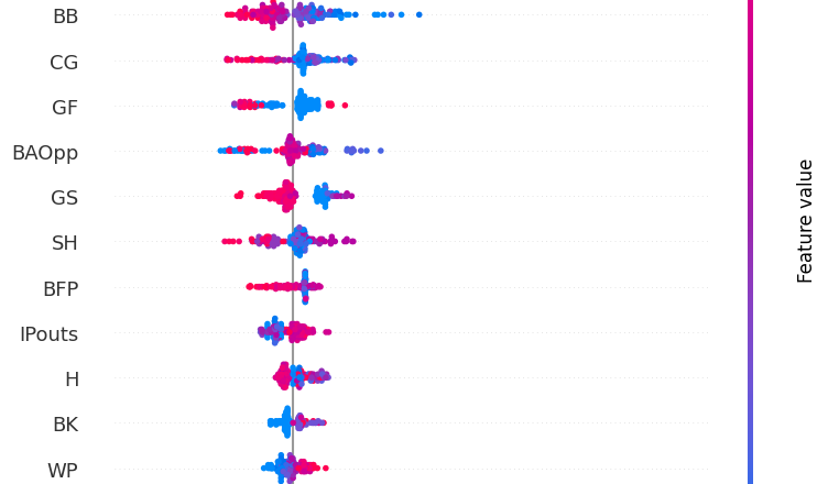
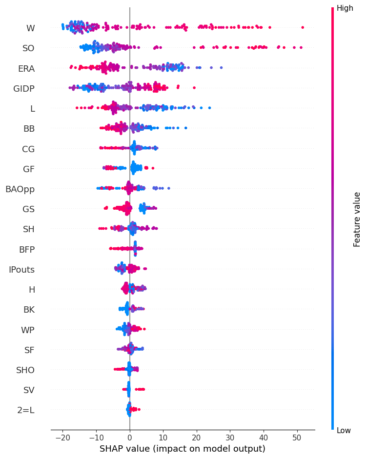
The below is a plot of LightGBM’s SHAP values for the testing data. A discussion of a few features should hopefully make the interpretation clear. Let’s take wins (W) for example. A higher number of wins (red dots) oftentimes drives up points won. This makes sense. Likewise, a lower ERA (blue dots) tends to increase points won. Again, this makes sense. Our model is making sensible choices.
Conclusion
Our goal was not necessarily to build the best possible model. To do so, we would need to try more models and engineer additional features. Rather, we wanted to lay out a framework for training models. Hopefully, you find it useful and inspiring for your own work.